AGP|CGM|See more..to judge better

AGP is a universal representation of diabetic patient readings over a specific time period in a way that we became enable to extract hidden pattern and glycemic information related to the patient behavior and treatment impact upon his case progression

Before we start lets examine this article / course which was developed by Prof.Roger Mazze and Dr.Iain Cranston:

all the the below explanations are taken from it and and viewed from various angles .....

What is AGP ? (ambulatory glucose profile )

it is a representation of selected glucose reading in a way as it occurred in single day .

upon smart analysis ;this representative enabled us from identifying various glucose parameters like glycemic variability ,hypoglycemic risk /episodes and glucose exposure

AGP includes two parts :

1-Graphic

and,

2-Quantitative

* Developed by Drs. Roger Mazze and David Rodbard,with colleagues at the Albert Einstein College of Medicine n 1987

AGP was initially used for representation of episodic self-monitor (SMBG). The first version included a glucose median and inter-quartile ranges graphed as a 24 hour day. Dr. Mazze brought the original AGP to the International Diabetes Center (IDC) in the late 1980's and since that time, IDC has built the AGP into the internationally recognized standard for glucose pattern reporting

important tip:

1-AGP should Not replace HBa1c while assessing glycemic status,Both should be considered .
for example :Glucose exposure could be evaluated by looking over HBa1c and glucose arithmetic mean/average

2-AGP is similar to ECG (heat electrocardiogram); universal approach of representing multiple/ unbiased/selected glucose readings in meaningful way

* Interpretation :

Using AGP score cards :

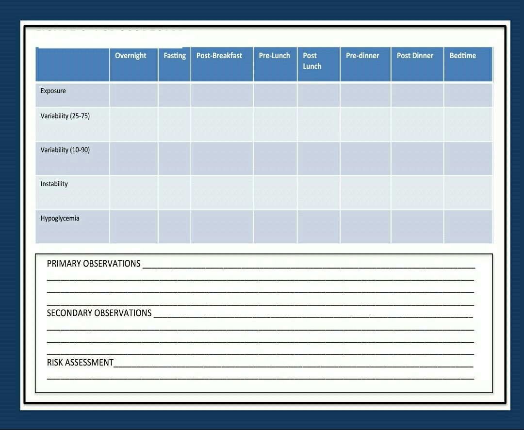
ٍSystematic approach used to assess five categories * :

1- exposure

2-variability (25-75)

3-variability (10-90)

4-instability

5-hypoglycemic

Those categories will be assessed along 7 periods:

1-overnight

2-fasting

3-pre launch

4-post launch

5-pre dinner

6-post dinner

6-bedtime

(More elaboration later ... )

AGP in brief vs Glycemic variability

Now,lets summarize this AGP core curriculum taught in AGP academy,Portsmouth,UK ...

in my opinion comprehensive digestion of this article is considered initial/step toward Frequent Pattern Management (FPM)

This course was developed by Prof.Roger Mazze and Dr.Iain Cranston:

since, the advent of CGM and FGM (called intermittent CGM,explained earlier) we become able to attain huge amount of data/readings which occurred in various periods of the day.
collapsing of these data together as it occurred in one day called AGP which enabled us -if plotted- properly to analyse glucose readings and discover hidden pattern of glucose excursion .
moreover ,individual glucose profile of each day (explained later) also could be plotted in order to be compared with the overall AGP for the sake of identifying frequent/infrequent patterns ...keep in mind that daily profile should be accompanied with Carbs. intake and insulin doses for better assessment of: glucose exposure ,glucose variability stability hypoglycemic and hyper glycemic risks
just to reiterate,years ago glycemic control was assessed against one figure like Hab1c or AVG regardless variability where complications MAY develop faster in person with frequent dysglycemia
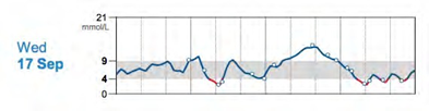
imagine a diabetic person monitors his blood glucose via normal SMBG ,three times a day; mostly-within the daytime if connected,mostly glucose will be in the target (4-9) however this is how the graph appears;
if CGM is used :

the CGM plot suggests a completely different diurnal glucose pattern. It shows periods of daytime hyperglycemia and mid-morning hypoglycemia undetected by the SMBG values.

since the representation of glucose values could differ from day to day,numeric estimation could be a solution: like Hba1c and AVG which may reflect glucose exposure and SD ,Delta waves(change )may indicate level of dispersion and variability/stability however due to certain limitation and inability to discover the underling causes of these abnormalities ,other approaches are adopted,so
80% of readings were plotted (collectively) in one graph so we can identify :

glucose exposure
intraday variability (stability )
interday varvariabilty
hyper and hypo pattern evaluation

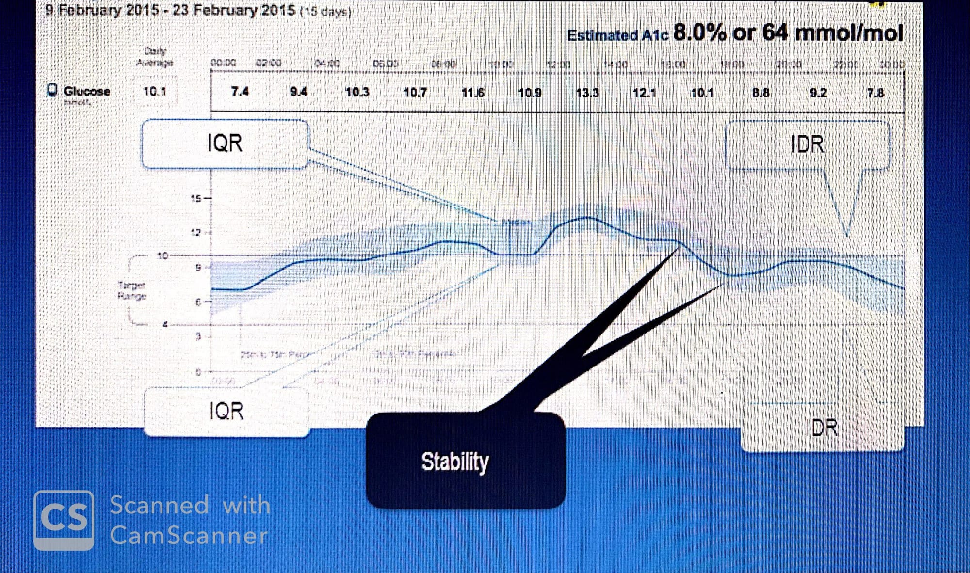
AGP with Inter-quartile and Inter- deciles Ranges

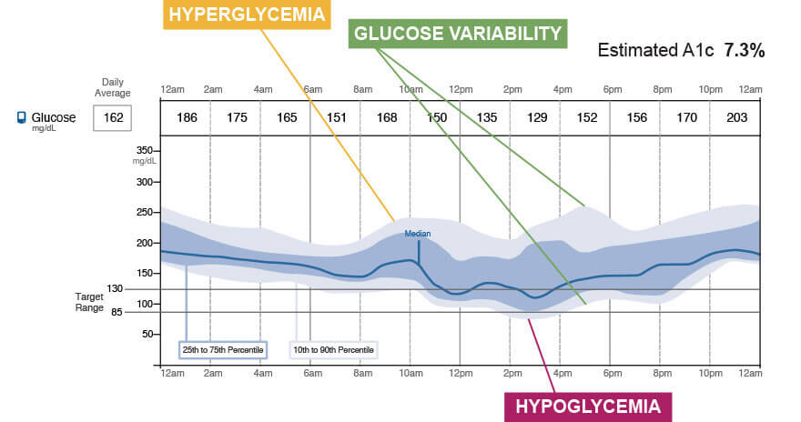
The center curve is the median. The darker area surrounding it, bordered by the 25th and 75th percentile curves is the inter-quartile range (IQR) and the lighter area bordered by the 10th and 90th percentile curves is the inter-decile range (IDR)

I will not go into details how to calculate the above parameters (AUC ... and integration )

since this not our main target but there are important insights can be got from this graph:

1- lack of symmetry which indicate that glucose readings were not equally distributed (this is could be normal and imply inter day variability

2-meaningful insights extracted from the graph by just-glancing without reviewing numeric parameters could be misleading !

3-in general 80 % of readings can give us an approximation of glycemic status -given that 20 % represent outliers !

4-the hallmark of AGP Representation is to simplify the pic. and diminish the vagueness

5-AGP gives an approximate overview of the last 14 days but when comparing it with individual which daily graph ;we can identify specific pattern if exist then underling causes of any deviation (more elaboration later.. )so this why its so important to examine both reports so each one can explain the other.

i.e AGP is like a general word and daily graphs are the letters which constitute this word....

* in order for AGP to be useful it must predict future outcomes through careful analysis of retrospective data :

many studies were carried on by (xing and other scientist)aiming to compare 3.7.14 days of CGM with subsequent 30 ,90 days .. without going into details . 3 conclusions were got :

14 days is the best period studied which has closest prediction of future patterns...provided there is a consistency in daily activities; however < 14 days could be enough in case of less variability
" a research of all pubmed- related citations) regarding CGM use in clinical practice, an international group of experts in diabetes care and research concluded that, “A minimum of 14 consecutive days of data with approximately 70% of possible CGM readings of those 14 days appears to generate a report that enables optimal analysis and decision-making" also,
" 12–15 day period of monitoring every 3 months may be needed to optimally assess overall glucose control.”

AGP could be perspective if it was generated retrospectively.....

nice example ...

1-Patent with 50 % basal insulin and 50 % bolus revealed the following AGP :

2-Upon careful examining ,his physician noted that a night hypoglycemia and post breakfast glucose variability so the endo. advised with less basal insulin and re adjustment of bolus insulin according to carb. intake ;examine his AGP after these amendments reveled reasonable improvement :

Note that HbA1c did not change albeit obvious improvement in AGP !! this real value of AGP and we need to review it along with HbA1c

Golden rules of AGP predictability :

1-14 days are standard but fewer could serve if high stability and less variability....

2- < 14 days could be beneficial but depends on what there are used for :

as perspective for the upcoming 30/90 days or just a surveillance monitor of a sudden change ..?

(According To Xing and his associates 14 days is a must to quasi accurate in our prediction for the next 30 days)

3-General consensus has been built regarding the AGP in order to be adopted by HCP :

i- American Diabetic Association (ADA)

ii- European Association for the Study of Diabetes (EASD)

3-In February 2017, at the Advanced Technology and Treatment for Diabetes Congress experts from academic centers in research, clinical care and patient advocacy prepared a consensus related to the utilization of continuous glucose monitoring. The results of the meeting were reported Diabetes Care. The report stated that, “…the AGP approach … is recommended by this consensus group as a standard for visualization of CGM data..."

“The Ambulatory Glucose Profile (AGP) … could be adopted to standardize summary metrics among devices and manufacturers. inter-quartile range (IQR) and area under the curve (AUC) should be used to represent glucose variability and exposure, respectively"

"Together, the graphic display and the quantitative data provide a comprehensive overview of diurnal glucose patterns that, in turn, are the basis of clinical decision-making. The use of a common reporting structure can contribute to the efficacy of CGM technology as it becomes possible to use different devices and employing a standard report, compare data"

As mentioned above ;5 parameters need to be evaluated once examined:

1-glucose exposure

2-variability

3-stability

4-hypo

5-hyper

but how ??? lets see ...

Glucose exposure :

Usually, as its measured-mathematically- as area under the curve - AUC using trapezoidal rule .

considering the each block as trapezoid and calculate it area (limited integration ) see below:

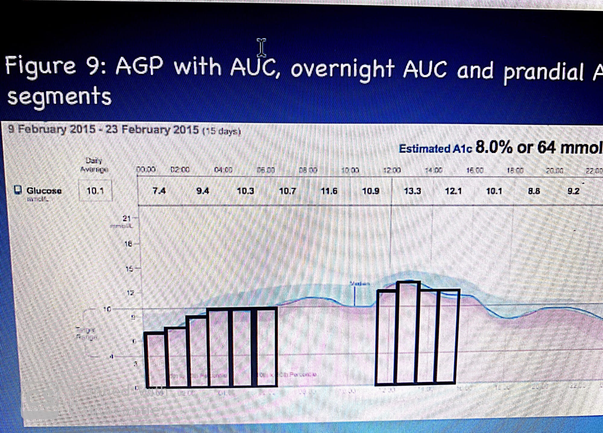
Thus, 𝐴𝑈𝐶 = ∑_{i=0 up to 24 i * P50i}

where i = hour of the day and P_50i = smoothed 50th percentile value for the hour of the day. Since the smoothed median values for each hour are expressed in mmol/L, the AUC is reported as mmol/L/24hrs

Imagine.. The area under the 25th percentile curve is 40 mmol/L/4 hrs; while the AUC at the upper limit of the IQR (the 75th percentile curve) is 53 mmol/L/4hrs; thus, the prandial range would be expressed as 40-53 mmol/L/4hrs. Note that the differences between the median curve and the two IQR segments are asymmetrical with the upper segment 60% larger than the lower segment. Providing further evidence that glucose is not normally distributed and varies from day to day. In fact, using the mean would be a misrepresentation of the diurnal glucose pattern. It would be suggesting that glucose is normally distributed and that the mean and standard deviation represent both the central tendency and dispersion of glucose values over multiple days.

In summary,

Glucose exposure -by the aid of glyculator ,it can be calculated easily-

however -alone- as we had seen above ; could be misleading -because of diurnal variability there is a clear difference between median curve and 75 percentile curve comparing the median and 25 percentile curve ,so there is a further reason why we need to consider other parameters -(mean and SD could be unhelpful ) in order to evaluate glycemic status --properly-.

Variability and Stability :

variability: refers to inter day variation ( Glucose variation from day to day )

Stability : refers to intra day variation (Glucose variation within the same day )

As per studies, done before there is a link between glucose oscillation and micro/macro diabetic complications

The average IQR is measured as the sum of the differences between the 75th and 25th hourly percentile values divided by 24.

The average IDR is determined by subtracting the 10th percentile hourly values from the 90th percentile value. The sum of the hourly values divided by 24 .

however, IQR and IDR could be misleading because glucose space between median and 25 percentile is not similar to the space between median and 75 percentile and the same thing applied to IDR

The median of the same AGP represents the average stability for each day. If each day were plotted separately and the plots were then accumulated using a best fit curve the result would be the median of the AGP. Stability is determined by summing the absolute difference in the consecutive values that comprise the median and dividing by the number of values( S[t₁-t₂ … t₂₄]/n ).

if IDR is higher than IQR ;This might suggest that the patient’s meals vary in timing and carbohydrate content and that the medication is not adjusted accordingly since :

IDR reflects the variability in patient behavior while;

IQR measures the effectiveness of the pharmacologic agent used to target post-prandial glucose levels

See the above figure where IDR is wider than IQR....for that reason.

As nutshell,

precise numbers are so difficult to be obtained ,so we are focusing mainly on their general impact in addition to other glycemic parameters -later we will see how to be analysed systemically .

Dysglycemia :

One of the major AGP insight is its ability to highlight the underling cause of hypo/hyperglycemia

through differentiating between patterns and episodic events. in order to prevent an over- reaction to outlier values ;AGP highlights the IQR/IDR. This is not to argue that the 10% values below or above the IDR are unimportant. It is simply to point out that the major trend is that glucose levels remain within the target range and that outliers need to be treated as anomalous values.

nice example..

In the AGP of the panel there is a pattern of hypoglycemia (mainly overnight and and most of the day)so Insulin has been decreased which leads to an improvement in the overall hypoglycemia but o-on the other hand -as seen in the other panel ,risk of hyperglycemia has been increased from (20 up to 65 %) .there is an overall shift toward hyperglycemia .

AGP is considered as risk analyzer to examine the hidden pattern but in order to discover the significance of outliers ;daily profiles need to be examined ..

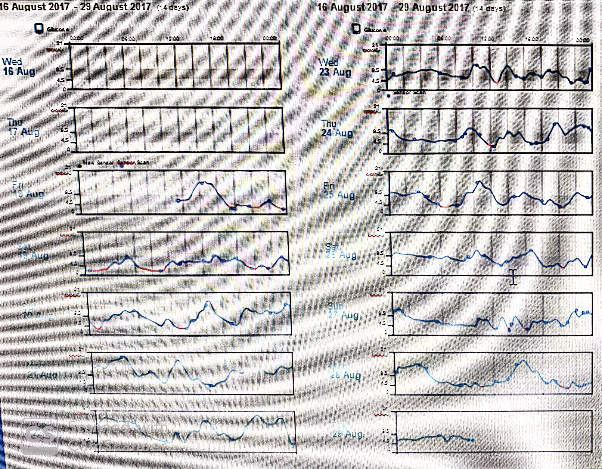
Both are AGP and daily profiles of each day constitutes the AGP for the same person taking basal and bolus insulin ...

*The overnight values show both hyper- and hypoglycemia, although the hyperglycemia appears more prevalent and problematic. During morning and evening glucose levels dip below the lower target.

* there is glucose excursion in postprandial period ,The hyperglycemic values and hypoglycemic values are generally found in the IDR and thus may suggest that they are relatively infrequent.

This raises several questions: (1) were these events anomalous; (2) did the patient experience any difficulties; (3) was there a clear, preventable cause; (4) are these events likely to repeat themselves?

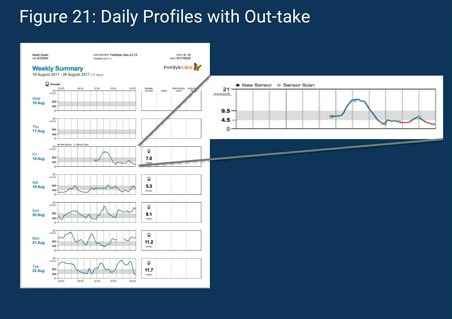
* Examining the daily profiles, is it possible to use one day to predict the next?daily profiles figure shows where and when these extreme values occur....

For example, on Saturday, August 19th there were four hypoglycemic episodes (shown in red), one occurring overnight; on August 20th, there is another overnight episode. These are indicated in the IDR as relatively infrequent because over the next 10 days they do not occur again. Reviewing the AGP with the patient by looking at the overall pattern and then the individual days, is the best method for discovering the answers to these questions. When the AGP and the individual profiles are examined together, values of concern can now be seen in relationship to when they occurred and the risk of being repeated. On August 21st, the overnight glucose values rose to near 21 mmol/L and on the next day to near 19 mmol/L. This was repeated on the 28th. In all three instances, the glucose levels returned to baseline by 08:00 hrs.

*What do these patterns signify? On the daily profiles, it was clear that there was an initial major hypoglycemic incident occurring during the first 24 hours of flash glucose monitoring. The low glucose began in the evening of August 18th following an episode of hyperglycemia. One can suspect that the hyperglycemia was over-treated. The common consequence of which is a sudden sustained drop in glucose. Between 14:00 and 16:00 hrs glucose peaked and was apparently treated with rapid acting insulin. This caused a sudden and sustained drop of 6 mmol/L in 3 hours. This is known because on the report it shows at the peak a small circle which is indicative of passing the reader over the sensor. The next time this occurs is when the glucose reaches 3 mmol/L. This suggests some action was taken, which is corroborated by the sudden slight rise in glucose into the target range. The over-treatment, however, overcomes this and reverses the glucose to move back into the hypoglycemic range. The hypoglycemia continues into the overnight period until 02:00 hrs when it reverses again. It appears that at 00:30 hrs. the patient again passed the reader over the sensor due to the low glucose levels and acted. Soon afterwards, there is a sudden excursion into the target range. However, whatever the remedy did not last, and again glucose dropped into the hypoglycemic range. This volatility appeared to be resolved by 10:00 hrs. This pattern repeats itself on the evening of the 19th and into the early hours of the 20th. Once again there is an over-reaction both when there are low and high blood glucose levels. This is mostly reflected in the IDR. Not until August 23rd does it appear that the glucose levels stabilize

* in order to assess various glycemic abnormalities ,we need to to see how AGP may look like of non diabetic individual :

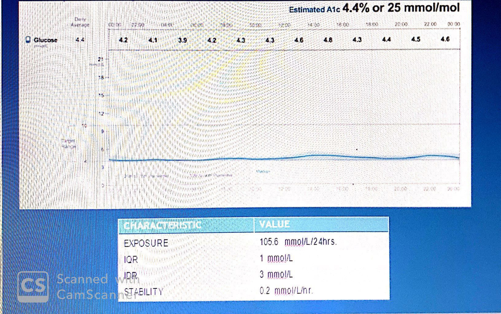this figures illustrates how effective the body is at maintaining homeostasis in the presence of sleep, wake, fed and fasting, activity and inactivity. also,individuals with normal glucose tolerance share several important AGP characteristics: (1) stable glucose levels, (2) minimal variability, (3) a small percent of values within the hypoglycemic range.

usually,glucose in normal person tends to hover around hypoglycemia threshold as seen....

so as we are mimicking this natural homeostasis mechanism of our body; glucose can be controlled tightly

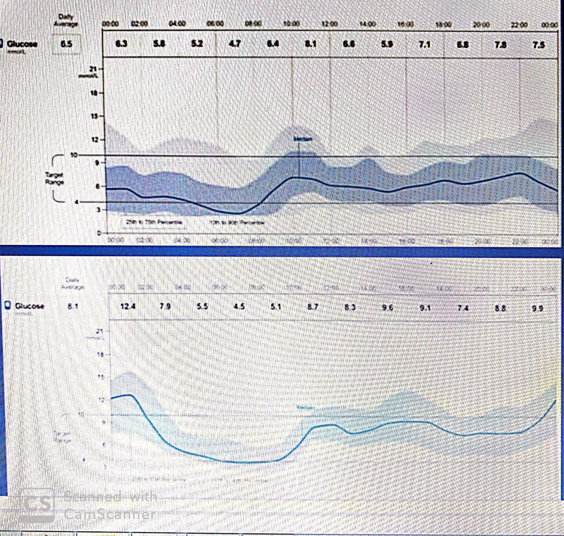
i.e our aim is to make diabetic AGP similar to normal AGP.. now lets examine these three AGPs who are using flash glucose monitoring :

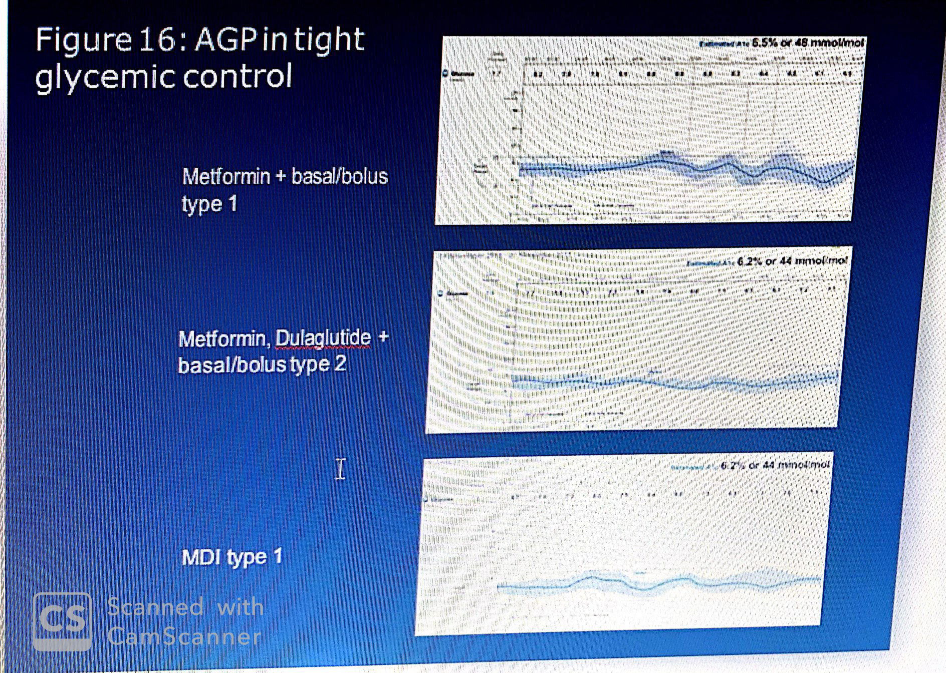
The top AGP shows meal related excursions generally within the target range for which the current therapy and/or diet were sufficient to stabilize glucose levels at 6.5% estimated A1c. Note that each excursion is followed by a sustained decrease in glucose only to be followed by another excursion. The pattern suggests that the basal/bolus regimen is synchronized to the diet. I

The middle AGP is of a patient with type 2 diabetes. It demonstrates the unique benefits of a GLP-1 receptor agonist (Dulaglutide) in terms of restoring glucose homeostasis. The GLP-1RA mimics natural incretin action, which is often found to be suboptimal in type 2 diabetes. Because it is administered once-weekly, essentially there is a constant circulation of this critical glucose sensitive artificial hormone. Only when glucose levels reach approximately 4.5 mmol/L does it cause the pancreas to increase insulin production, while simultaneously reducing excess hepatic glucose production and slowing absorption of food. This combination of actions tends to reduce variability and stabilize glucose levels, especially when used in combination with insulin.

The lower panel AGP is of a person with type 1 diabetes treated with evening basal and pre-meal rapid acting insulin. The patient was taught to use an insulin to carbohydrate adjustment factor for insulin dosing prior to each meal. It illustrates the impact of this approach on glucose control following both mid-day and evening meals. Note how the IDR at mid-day and the IQR at dinner show wider variability. This indicates that both the inter-day meals vary and that the current “adjustment” algorithm is inadequate. The benefit of isCGM with AGP analysis is that it permits a dynamic process in which the AGPs identify underlying problem areas whilst also suggesting where to focus possible remedies. In this case, it suggests that the response to mid-day meals requires a behavioral intervention while the response to evening IQR requires a reconsideration of how/when insulin is dosed.

* As mentioned above, AGP represents two parts : quantitative (metrics) and qualitative (graphic),

Both should be considered in order to -accurately-assess the glycemic status -considering only one could be misleading as we will see...

Note: Xcel software can be programmed to make the calculations, if the proprietary software accompanying does not make the calculations. All CGM data are organized by value, date and time. They can be imported from the reader memory and transferred to an Xcel file format.

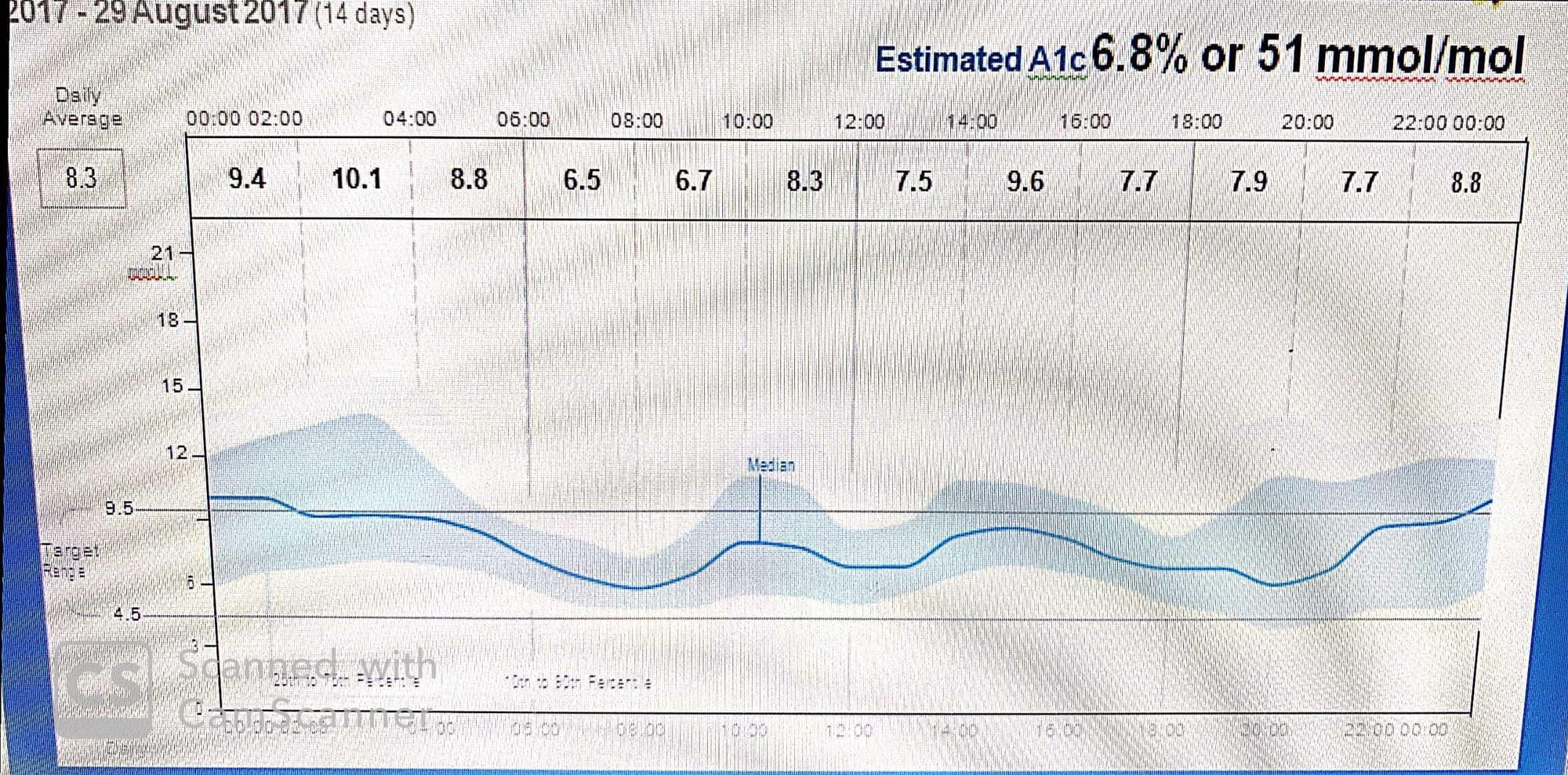
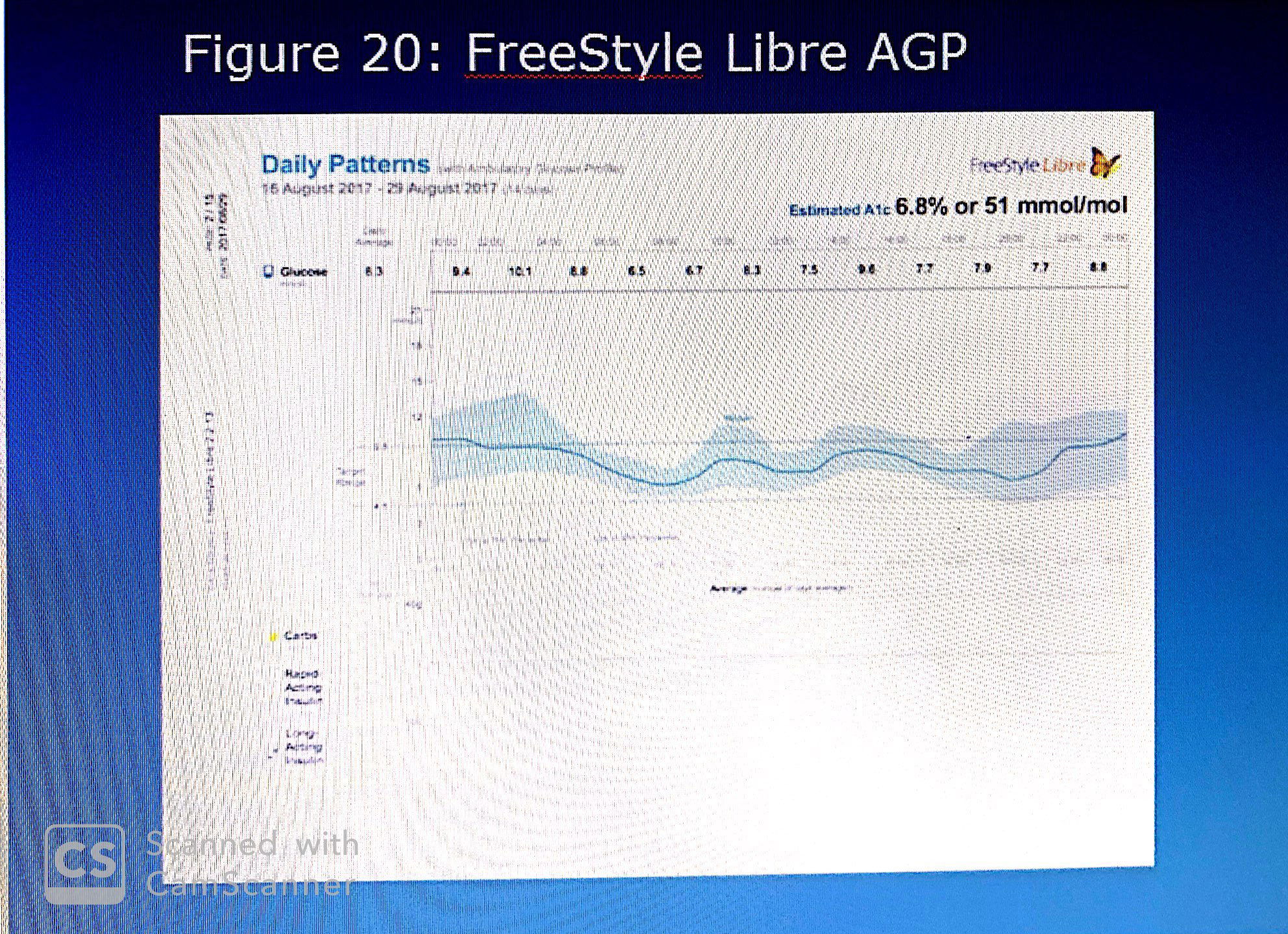
the quantitative data that can be derived from the AGP. It also shows the daily profiles. Together this presents a comprehensive assessment of glycemic control. Taken separately,SPECIAL NOTE: Figure above, was produced using FreeStyle Libre software which reports the overall average glucose (left side) and the estimated HbA_1c (right side). The average is calculated using the raw glucose data and the estimated HbA_1c is determined using the Nathan formula for conversion from HbA_1c to estimated average glucose: 28.7 X A1C – 46.7 = eAG. For calculating the “estimated A1c”, the formula is: [(Average in mmol/L x 18) +46.7] /28.7= estimated HbA_1c. Because the formula uses all glucose values, when patients have a significant number of glucose values in the hypoglycemic range the estimated A1c will read lower than the laboratory value. Additionally, the graph reports the average glucose for each two-hour interval:

Partial assessment that can be misleading:

Note, for example that the AGP and the quantitative data complement each other:

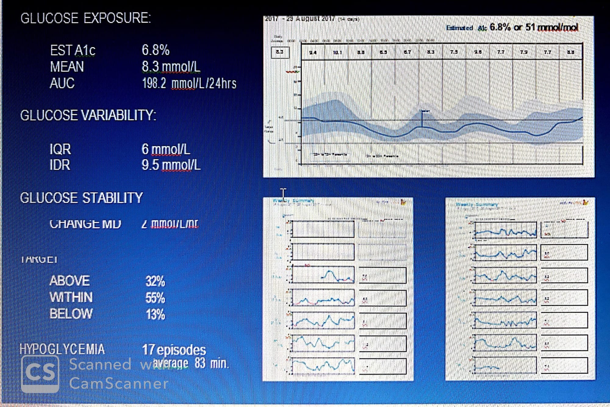
1- Without the AGP, the estimated A1c of 6.8% suggests tight glycemic control; however, with the AGP glucose variability clearly presents a problem in management. AUC denotes 91 mmol/L/24hrs excess glucose exposure when normal exposure (106.5) is subtracted from current exposure.

2-Interestingly, although the quantification of stability, 2 mmol/L/hr, does not appear significant, examination of the daily profiles gives a different picture. Compared quantitatively, it is almost 10 (0.2*10=2) times less stable than normal. Of significance is the incidence of hypoglycemia. The AGP identified 17 episodes (at least 10 min <3.9 mmol/L) each lasting an average of 83 minutes. The AGP shows that overnight, mid-day and evening are all problematic periods. The individual days show in red on the profile exactly when these events occurred.

3-Thus, it is incumbent that both the qualitative and the quantitative data must be taken into consideration when considering initiating treatment, adjusting therapy and, most important, actively intervening to improve glycemic control through behavioral changes. It has been argued that patients hold 95% of the information upon which physicians make their decisions in diabetes. Flash glucose monitoring (or isCGM) with AGP analysis obviates much of this information. Evidence-based medicine is guided by the principal that the information upon which decisions are made be unbiased, accurate and reliable. Continuous glucose monitoring with AGP analysis assures that patient generated data meets these criteria.

4-FSL reports aim to represent collected data in understandable way (visual picture which donate to any abnormality within the AGP ) with less attention to the numeric figures obtained from AGP due to two main reasons :

a-those figures are easily calculated by any software

b-those figures could be misleading and add complexity to AGP interpretation

Brief :

* All CGM systems use a sensor approximately 5 mm in length placed under the skin in the interstitial fluid connected to a transmitter sitting on the skin surface. The sensor is coated with glucose oxidase that catalyzes the oxidation of glucose converting the reaction into an electrical current which is either stored by the transmitter or immediately sent to a reader.

* Transmitter (sensor ;the same !; capacity is 14 days in flash glucose monitor while it has no memory in CGM .data-contentiously- transferred to the reader via Bluetooth . Whether continuous or intermittent, the transmissions are wireless.

* Because the sensor is placed in the interstitial space its measurement of glucose differs from simultaneous measurement in blood. Interstitial glucose (ISG) is the result of glucose in the blood stream being transferred into the interstitium via passive diffusion.

* The interstitial fluid (ISF) bathes and surrounds all cells/tissue. When the volume of glucose in the blood stream (capillary system) is greater than in the ISF, the glucose migrates into the ISF. From the interstitial fluid, the ISG (with assistance from insulin in insulin dependent tissue) moves into the cell.

*Thus, glucose passes through two barriers to reach target tissue. This suggests that there are three different glucose concentrations: in blood, in interstitial fluid, in target tissue. Measurement of glucose reaching target cells has been based on glucose measured in blood either using a laboratory assay or self- monitored blood glucose taken from capillary samples. Both low and high glucose levels are deemed detrimental. Therefore, virtually all changes in treatment are blood glucose dependent. This assumes that, for example, when blood glucose is low, increasing carbohydrates will benefit glucose levels and thus make more glucose available to target tissue. When glucose is too high, added insulin and exercise are often used to restore normal levels. However, in most cases this ignores the issue of the two barriers between capillary beds and interstitium and between interstitium and target cell. Thus, blood glucose levels, such as SMBG are used as the surrogate.

* A major problem arose with the introduction of interstitial glucose (ISG). What was to be done about the effect of the barrier on glucose level differences? The easiest solution was to continue to use blood glucose levels by re-calibrating the interstitial glucose to blood glucose. The process was simple. Take a sample of the blood glucose (SMBG) and simultaneously measure the ISG adjusting the value to match the SMBG value. It was quickly found that while during times of steady glucose levels this worked well, when glucose rapidly ascended or descended the values differed by between 15 and 20%.As glucose rises in blood its concentration increases and thus causes the passive diffusion into the interstitium. But there is a delay in this process. Essentially the glucose is higher in blood than in the ISF. The difference is now used as the calibration factor, all subsequent glucose values are now recalculated to account for the difference. Not until the next calibration, is there a change in the calibration factor. As glucose descends the reverse takes place, consequently glucose may be lower in the capillary blood than in the ISF. Considering these factors, the difference in glucose value between SMBG and ISG simultaneous samples could be as little as 0% to as great as 17%. The differences are time sensitive. If glucose in the blood moved quickly into the ISF the lag would be an insignificant factor. However, the time lag ranges for from five to fifteen minutes. The difference can be significant if real time glucose levels were guiding clinical decisions, especially under conditions of rapidly changing blood glucose.

To mitigate this, CGM device manufacturers use calibration to blood glucose combining the simultaneous measures with proprietary algorithms. The patient uses SMBG to obtain the current reading and enters this value into the CGM receiver. The receiver uses the algorithm to re-adjust the current CGM reading; consequently, the greater the number of calibrations the more accurate the CGM reading when compared to SMBG. Thus, current CGM devices require four or more calibrations each day. The proprietary algorithm needs to consider the time lag and value differences. Because the time lag may be a problem for patients dependent upon real-time blood glucose levels to control insulin administration either by pump to multiple daily injections, and because CGM devices sound alarms when glucose levels reach low thresholds, accuracy has become a major issue with regards to routine use of CGM for clinical decisions. Additionally, because the calibration values are entered manually they rely on the accuracy of the SMBG meter, the patient’s skills to obtain the SMBG sample and entering the correct value. Consequently, utilization of CGM for real-time diabetes management has become problematic.

* In 2014, a new form of CGM was introduced. Called flash glucose monitoring, it uses the same chemical glucose oxidase mechanism for glucose measurement as CGM with updated wired enzyme sensors incorporating osmium. Because this sensor technology does not produce as much “drift” as earlier sensors and has a more stable response over time in glucose measurements, it can be calibrated at the time of manufacturing and does not require re-calibration by the patient. A second innovation is that the new technology allows the sensor to stay in place for up to 14 days.

* How does the factory-calibrated system compare to a patient-calibrated version? When patients simultaneously wore the flash glucose monitoring system with factory calibration and with patient calibration the difference in glucose values were negligible, but favoring the factory calibrated system.Thus, when tested against standard CGM these innovations are more closely correlated to blood glucose measured simultaneously. How is this possible? The sensors are calibrated against blood samples in the manufacturing process, consequently each batch that is produced has the same adjustment to blood glucose. It has been reported that since glucose levels change throughout the day, how can one calibrated value suffice? Since the introduction of CGM there has been an intrinsic problem with SMBG-based calibrations that was essentially overlooked. Manufacturers assumed that patients would frequently monitor their blood glucose and correctly enter the calibration into their CGM devices using SMBG meters that were constantly being re-assessed for accuracy. In practice, however, patients skipped SMBG, inaccurately entered calibration values and used outdated or error-prone SMBG meters. In short, the patient calibrations were subject to significant error.

These skilled-based and meter-based errors led to greater variability than factory-calibrated sensors. In additional, the wired enzyme technology made for a more stable and consistent measurement, thus reducing the likelihood of sensor-to-sensor variability.

* Another significant difference between standard CGM and flash glucose monitoring is how the information is stored, transmitted and reported. As previously mentioned, rtCGM sensors constantly measured glucose and pass electrical signals to the transmitter (worn on the skin surface), which converts the electrical current to a format that could be continuously transmitted to a nearby receiver. The receiver stores the data in a manner that could be uploaded to a computer which, using proprietary software, aggregates the data into a series of reports. Due to the proprietary nature of the software the reports are not comparable among manufacturers. Some companies accumulate the data in five-minute intervals while others use ten-minute intervals. Thus, based on the manufacturer, the graphic displays could have as many as 288 points for a single day.

* Flash glucose monitoring or isCGM uses a novel approach to capture, store and report glucose data. To understand this best, it is important to know that unlike rtCGM devices, the flash glucose monitoring receiver (reader) functions to capture sensor data only when the user scans the transmitter using a special reader (which can be a phone application).

Suppose, however, that the user of the receiver is not the patient, but a health care professional; wants to understand the typical diurnal glucose patterns of a patient before initiating therapy with minimal patient bias. To accommodate the professional user, a second flash glucose monitoring system was introduced. A similar sensor and transmitter are used. However, the transmitted can store 14 days of data and the patient cannot see these data: called Freestyle libre pro :

FREESTYLE LIBRE PROFESSIONAL FLASH GLUCOSE MONITORING

The professional version of flash glucose monitoring (isCGM) is very similar to the personal version in terms of its collection of glucose data. However, it differs in two very important ways:

First, the 14-day sensor worn by the patient does not require an 8-hour reader. Essentially, the 14 days of glucose data are stored in the transmitter and are “blinded” to the patient. .

Second,The professional reader can be used on multiple Libre Pro transmitters, thus only one is required. Similar in design to the personal reader, the professional reader can collect data at any time from a patient wearing the special transmitter.

Also, ibre pro could be used by HCP for diagnosis purposes (discussed later )...

To start with ....

AGP viewing is paramount since :

1-it will enable us to distinguish between real hypoglycemic episodes (glucose < 3.9 mmol/l)

and rapid descent of glucose from (18 to 8 mmol) :relative hypoglycemia ;both produce the same symptoms like shaking and malaise but different action maybe required.

2- examining three important reports needs to be examined -carefully-:The Snapshot provides a quick view of the AGP, episodes of hypoglycemia and data sufficiency. The Daily Pattern is the AGP. The weekly summary contains the daily profiles which together constitute the AGP ( SDW).....

One of the most important outcomes of AGP analysis is determining the priorities of abnormalities : variability,stability and hypo/hyper glycemia in order to figure them out -if present- and address them accordingly .

with the help of continuous AGP analysis ,also,we can evaluate any intervention impact whether its therapeutic or behavioral till reach our optimum goal of diabetes management.

As the previous is related to to theoretical analysis of AGP,lets move on toward actual cases and learn how to utilize our knowledge for better understanding and management of diabetes ..

case 1 :

This is the case of a female, 28 years of age with type 1 DM for 18 years. Treated with basal/bolus insulin using a 50/50 ratio with adjusted rapid acting insulin before each meal. She presents with no complications and a laboratory HbA_1c of 7.0%.

I-her snapshot report:

five things are revealed :

1-Hba1c = 6.8 % is indirect measure of previous glycemic status (since its calculated value ,hypo. episodes may affect it , approx each 10 % causes estimated HBAc to be less by 1 % compared to lab.HBA1c

Actually this estimated HBA1c can be used to compare AGPs as it gives you implicit /relative value of previous glucose exposure

2-the mean (arithmetic average ) give you an overall picture of glucose previous data (remember glucose was not normally distributed )so its indication may not be accurate but relative measure .

3-the percentage of values:

here ,obviously, it will appear the importance of AGP interpretation : qualitatively and quantitatively :

above target = 32 %

within target =55 %

below target =13 %

However when you look to the AGP ,you will see those data are not equally distributed on the whole graph i.e the days constitute this AGP that some days have more hypo episodes than others i.e inter/intra day variability is captured .

Looking at the AGP to the right, the distribution of these values can be examined. Note that between midnight and 06:00 hrs it appears that almost half the values are above target and few values below, while between 06:00 hrs and noon most values appear to be in target, except for late morning when about 25% of the values are above target. This underscores the importance of interpreting data within the context of the AGP. Without the AGP it is impossible to detect the variability in the “target” data.

4-low glucose events :

since some of the hypo episodes are outliers (outside IDR ) they cannot be captured here (this snap shot includes 80 % of data ,only) but again it gives an idea of hypo episode and how many they lingered .

eps. last for 83 min. but nothing can be explored of why and when those episodes occurred unless daily profiles have been examined (discussed later )

5-data sufficiency : usually > 70 % is considered good collected data

In order to maximize this period we to need to scan the sensor every 8 hrs. during the whole sensor wearing period ..

in the above figure we can see the average daily scan = 8 scans/day but the percentage is still not high bec. either:

User did not scan each day or(skipped a day without scanning) ; or

Many scans were done in a day (less or more than 8 hrs apart )

But,to capture that -precisely-,daily profiles need to be examined..

Finally,At the bottom of the page is room for comments. Additionally, on the upper right side of the page there is a space for information (such as units of insulin and grams of carbohydrate) that the patient recorded during the 14 days of monitoring. however,

these entries need to be precise without false estimation ,also compliance is needed esp. at the time of insulin dosing ,otherwise the generated reports could provide unreliable data.so its important to note here that AGP still can be generated although carbs,insulin, are not recorded !

Again this will switch our mind to re think about the prediction algorithm used by FSL whether it is related to entries or rate of change or both! remember that the most important reports in AGP analysis is :

(SWD)....

II-daily pattern (AGP):

1-first of all, this AGP needs to be compared with normal AGP characterized by :

NORMALLY,glucose levels range between 4.0 and 8.0 mmol/L with an IQR of less than 2 mmol/L. The median tends to be flat and the incidence of both hypoglycemia and hyperglycemia negligible.

2-its -only- the AGP which can capture the hypo.pattern and warn that any clinical decision if taken to manage hyperglycemia could exacerbate hypoglycemic episodes

3-also,closer examination reveals that the IDR upper quadrant is wider than the lower quadrant suggesting that the range of high glucose (75th to 90th percentile) is greater than that of low glucose (10th to 25th percentile). Thus far, the overview has revealed hypoglycemic risk, wide variability and persistent hyperglycemia.

4-Glucose exposure assessment :

Simply we can refer to the average number in the box of each two hrs interval i.e.

Both graphically and quantitatively the period between 02:00 and 04:00 hrs indicates the highest exposure, while the period just before awakening (06:00-08:00 hrs) graphically and quantitatively indicates the lowest exposure

5-stability :

How should the stability be described? Stability is a measure of intra-day oscillations, as such it requires a criterion. Normal glucose metabolism is essentially without oscillations. What criteria should be used for persons with diabetes? One of the benefits of AGP analysis is that changes in glucose levels are easily detected by comparing one AGP to the next one. In this AGP, post breakfast and pre-bedtime show the greatest instability.:

" The two-hour values, however, have importance because they provide insights into the intra-day variability. Note, for example, that the difference between the second and fourth time periods is a 3.6 mmol/L drop, suggesting that before awakening the patient undergoes a significant decrease in glucose level. The glucose levels rise again in the next four hours and then oscillate until they appear to stabilize"

The next review is the integration of the graphic and quantitative data:

i-Because the estimated A1c is based on all the values and thus, unlike laboratory assays, is affected by the incidence of low glucose values, it is important to determine to what degree the estimated A1c is affected by the number of low readings. In this example:

there are two kinds of quantitative data to consider.: First, the incidence of hypoglycemia and second the definition of “low glucose”.

There were 17 incidents of hypoglycemia (<3.9 mmol/L) lasting an average 83 minutes. This represents less than 1% of the time in hypoglycemia.

Consequently, these values would have little quantitative impact on the average glucose value.

However, the low glucose report indicates that 13% of the time the patient is below target (4.5 mmol/L). Together this would suggest that 12% of the low values are between 3.9 and 4.5 mmol/L while this is a significant percentage, because the target itself is above the threshold for hypoglycemia, its impact on the estimated A1c would be negligible.

if there was a concern, a simultaneous laboratory assay would be indicated. If the estimated A1c is lower than a simultaneous assay and the period of 45 days prior to the assay was relatively unchanged in terms of therapy and behavior, it suggests that hypoglycemia is playing a significant role. Under all other circumstances the two values should be comparable.

6-Based on the above AGP-without hearing from the patient -we can recommend the following :

i-it would appear that the priority would be to lower the excess overnight glucose exposure. This would be accomplished by increasing the basal insulin. However, while this would lower the glucose exposure it would worsen the variability and likely increase the risk of hypoglycemia. The only way to reduce the excess glucose exposure without risking hypoglycemia is to first address the overnight variability. Since both the IQR and IDR are wide one can suspect that neither the basal insulin nor the current diet is appropriately synchronized to prevent hyperglycemia.

2-The first step would be to modify the pre-meal insulin and to examine the four hours following the meal to determine whether the insulin is adequately control the post prandial excursions

3-Second, to re-examine the diet to determine the glycemic affect. If the patient is consuming varying amounts of carbohydrates, but staying on a fixed insulin regimen, this is the problem. If the patient is adjusting insulin to account for carbohydrate content, then the algorithm is incorrect.

4-the third step would be adjusting the basal insulin to account for any residual glucose excursions caused by diet to overnight excessive hepatic glucose output. These three steps must remain focused on the variability.

5-Once overnight variability is lessened, the focus would move to reduction in overall excess glucose exposure as indicated by the postprandial excursions. To do this, daytime variability must be addressed first to prevent increasing the risk of mid and late day hypoglycemia as glucose exposure is treated.

6-Reducing postprandial variability requires differentiating between meal-related causes, such as carbohydrate loading and medication-related causes, such as inappropriate use of insulin in terms of timing and dose. Meal content and amount is a matter of patient choice whereas insulin timing and dose is often in the purview of the physician.

in general;

wider IQR means something wrong with insulin n timing

wider IDR means something wrong with meal composition ....

III-weekly summary:

examining individual daily logs can reveal important information which can not be captured by AGP alone :

Above figure shows the 7 days which constitute the AGP;the following can information can be obtained from the above diagram :

1-Examining the first two days resolves the earlier question as to the 79% reported values. (no scans in the first two days )

2- Since there are no further data gaps, it is assumed that the patient complied with the 8-hour scanning rule after the second day.

3- Looking at August 18th, the patient’s first scan occurred just before noon. Interestingly, the next series of scans occur two hours later and only after the glucose rose to its apex. The subsequent scans occurred only after the patient reached the lowest glucose level for that day. From that point forward there are a series of scans, no doubt due to the sequence of low glucose values (delineated in red). It is almost as if one were watching the patient as he/she tries to resolve the hypoglycemia. In this case, the initial correction seems to be effective between 20:00 and 22:00 hrs, only to decline again and continue to remain in the hypoglycemic range into the next day. This helps identify the two significant incidents of hypoglycemia reported in the low glucose panel in the “snapshot”.

4-The last three days of the first week show the widest inter-day variability. Note that overnight glucose levels rise on the 21st to 20 mmol/L while two days earlier glucose levels at the same time were near 4.5 mmol/L. At 14:00 hrs on two successive days the same phenomenon occurs. This confirms the earlier observations of overnight and daytime variability.

5-On each of the daily profiles there is substantial fluctuation (or oscillations) in the curve. This suggests that the earlier observation (based on examination of the AGP median curve) of relative stability was inaccurate.

6-The first five days show significant fluctuations in the daily curve that will need to be addressed in the treatment plan. On these days, scanning (reading glucose levels) appeared to occur at the peak and valley, and rarely during the times in which the glucose was rising or falling. This suggests that the patient was only reacting when values reached extreme levels. It points to a behavioral rather than medication issue.

7-On the 21st of August, there is a two-hour gap in the profile. This indicates that the patient failed to scan within 8 hours. In fact, the next scan occurred on the following day in the early morning hours. Looking at the five daily profiles it is also apparent that one day does not predict the next. This suggests that changes in the treatment regimen have to consider variability in medication administration, meal timing and content as well as sleep/wake patterns. What explains this variability and instability? The first week’s daily profiles provide some evidence that patient behavior is a key factor. It appears that responses to instability are delayed and over-compensatory.

Now,lets examine the next 7 days :

1-The profiles completed on August 23rd and 24th show marked improvement in overnight glucose stability.

" Note on both days just after mid-night the patient scanned the sensor. This might suggest a decision to act or not was made at that time" this issue needs be discussed with the patient .

2-. On the August 23rd the patient scanned three successive times beginning at 8:00 hrs. The consequence seems to be a dampening of the subsequent peak value. Is the patient “learning” to anticipate the direction of the glucose change and reacting? Again, only a discussion with the patient will resolve this question.

3-on 25th of August indicates that the patient still has difficulty reacting in sufficient time to change the course of the extreme glucose excursions. Just before 04:00 hrs the patient scanned and based on the subsequent decrease in glucose level into the hypoglycemic range, over- reacted. Based on the succeeding two scans that patient could not halt the decline. At between 06:00 and 08:00 hrs the patient acted, resulting in a steady increase in glucose level at a rate of 5 mmol/L/hr, the patient reached an apex of 15 mmol/L at which time another over reaction occurred causing the glucose levels to decline at a rate of 5 mmol/L/hr. These series of over-reaction to both low and high glucose levels suggest a need to teach or re-teach the patient how to react without over compensating and causing these wide oscillations.

Note that the mean glucose levels reported to the right of each profile provide little evidence of these significant fluctuations!!!! (another evidence that mean-alone could be misleading )

Golden conclusions extracted from the above two graphs:

Overnight and afternoon-evening risk of hypoglycemia—found principally during the first week and appears to be due to over-reaction to hyperglycemia.
Significant overnight glucose variability and hyperglycemia—found throughout although seems to moderate during the second week. The cause appears to be over- reaction to low glucose levels.
Significant pre-awakening glucose decrease—occurred because of reaction to overnight hyperglycemia.
Overnight excess glucose exposure—appears in part due to overnight experience with hypoglycemia
With the patient’s input, there is the opportunity to not only understand what has occurred but also to teach the patient how to use isCGM (F.S. Libre) to anticipate glucose levels and to take pre-emptive action.

Tip from prof.mazze :

It is advised to focus on the recorded data initially and to discuss with the patient insulin administration and meal content. When it is felt that the patient can accurately measure and report carbohydrate intake as well as precisely note the timing and amount of insulin, it is suggested that the AGP along with the daily profiles and the patient’s medication and carbohydrate recordings be used to determine whether the patient’s diet is being adequately managed by the insulin and non-insulin medications.

In general ,

daily profiles careful examination enables us from capturing exact times /underlying causes of any abnormality shown by snapshot report since this report gathers a accumulative information and represent them as summary but weekly report indicates individual variation /stability and dysglycemia risks based on specific dates/time and why they occurred and when rectified if this has been shown any time .

moreover ,weekly summary report examination encourages patient input and mutual discussion which will play pivotal role in any further amendments or interventions .

also weekly summary report can answer many questions and clarify any doubts or observations like gaps or unclear observations like continous dysglycemia

more than that ,behavioral changes and patient reactions(timing of insulin dosin/carbs intake and even scanning can be captured very well since a all are recorded in this report

finally,its much more better to examine this report alongside with AGP repot in the same time in order to find clues or reasonable justification of any abnormality observed on snapshot report

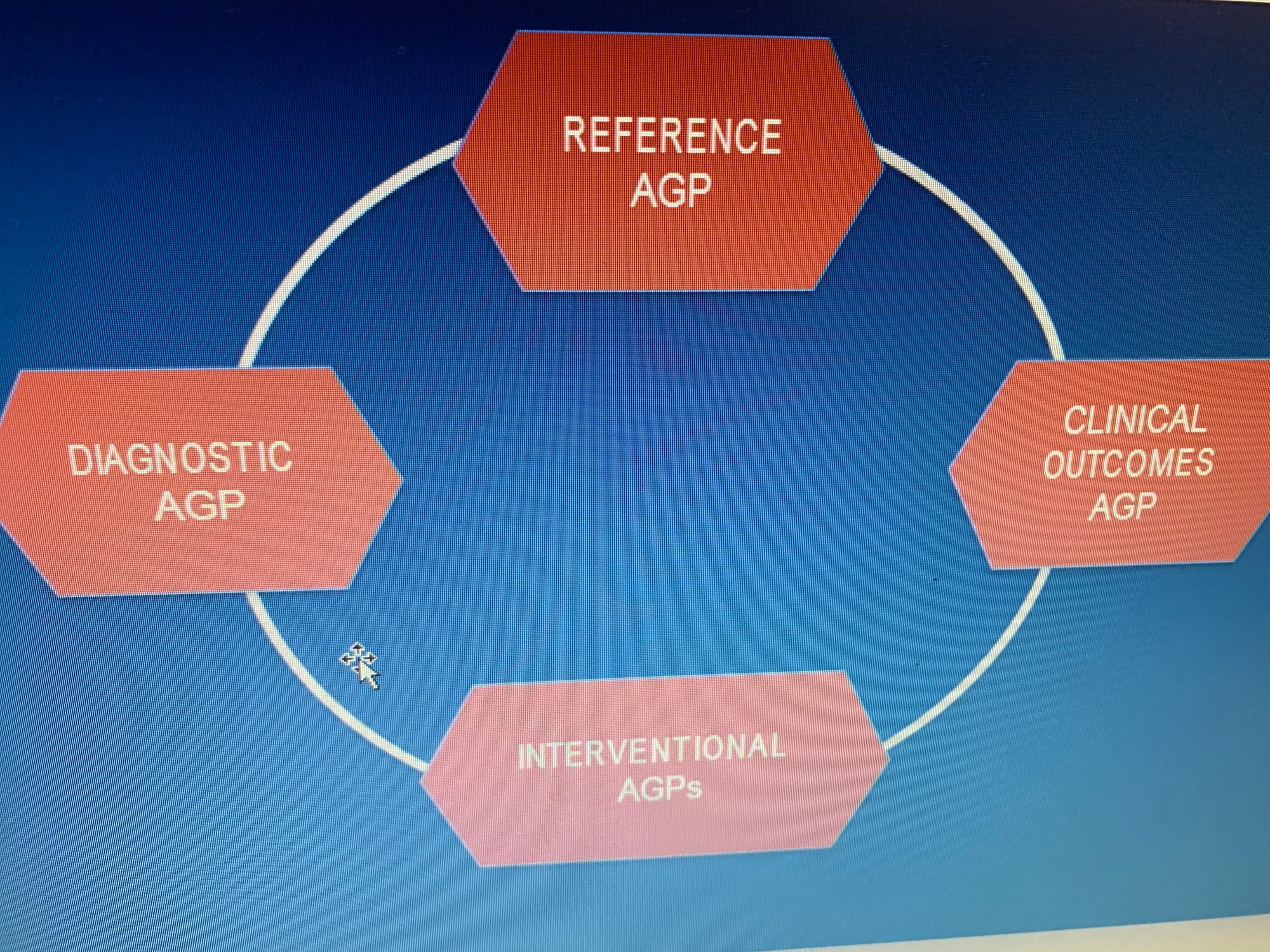
* AGP can be used/viewed from four angels :

1-reference :

is meant to serve as a baseline against which all clinical actions are measured. It asks the question, “What is the patient’s current metabolic status?” Essentially, it presents a “visualization” that should enable the physician to identify the dysglycemia. Unlike the HbA_1c, its importance lies in its specificity. Hypoglycemia and glucose variability cannot hide from the AGP depiction of the diurnal glucose pattern.

2- diagnostic :serves a very special purpose. The term pre-diabetes has come to mean individuals who appear to have risk factors associated with diabetes. Principal among this is the inability to adequately control blood glucose levels. Previously, terms like borderline diabetes, fasting glucose intolerance, and others were used to identify these individuals. Elevated HbA_1c and other measures were also used. However, these quantitative measures did not reflect the “conditions of daily living” that often exaggerated the underlying dysglycemia and went undetected. Diet and exercise, stress and inter-current which have a major impact on glycemia were often missed. With the advent of CGM and AGP analysis it is now possible to detect abnormalities in glucose metabolism with sufficient specificity to aid in the diagnosis of diabetes.

3-intervention : The intervention AGP focuses on the question, “What is the optimum approach to resolving the problem?”

4-clinical outcomes:The final use of the AGP is as a measure of clinical outcome. The current over-reliance on HbA_1c has removed specificity from discussions and measurements of clinical outcome.

Examples :

1- A 60 years old male with type 1 diabetes for 30 years presented with a recent HbA_1c of 7.3%.

2-Treated with multiple daily injections of basal (50%) and pre- meal bolus (50%) insulin,

3-The patient reported 6-7 SMBG tests each day with substantial viability in glucose level.

The physician, concerned with possible underlying hypoglycemia- initiated flash glucose

monitoring . He asked the patient not to change treatment, meals or activity during the two-week monitoring period

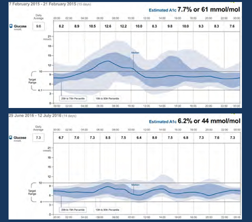
his current (reference/diagnostic AGP ) :

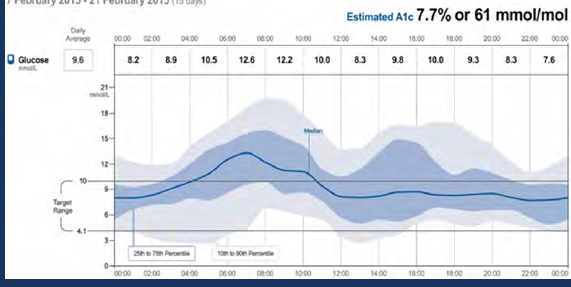
* two clear observations noted from above :

1- night hypo hypoglycemia

2-daytime hyperglycemia

so initially, the basal insulin (long acting) should be reduced ...

Prof.r.mazze :

An alternate means of obtaining a reference or diagnostic AGP is to use a blinded isCGM system. As mentioned in the earlier module, the profession version of flash glucose monitoring (FreeStyle Libre Pro) uses a blinded transmitter which stores data for 14 days. Only the physician can obtain the readings by scanning the transmitter with a professional reader.

* after clear intervention -one month later - lets see the AGP again :

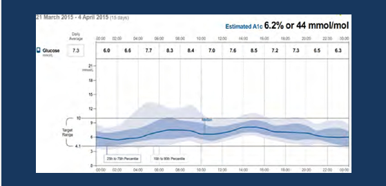1- HBa1C has been reduced by 1.3 % ( 7.7 to 6.2)

2-general reduction of glycemic variability : hypo and hyper

3-general improvement in postprandial glucose level (after eating ) which indicates patient increased awareness of eating habits

for further improvement ,patient was advised to proper snacks amount before sleep to avoid night hypoglycemic attacks ,after two months ,his AGP appears as below :

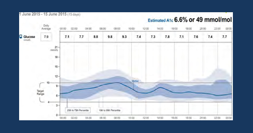
1-Stability did not change

2-over night hypoglycemia had been reduced

3-patient claimed hat he ate more snacks to avoid hypoglycemia

so his doctor -slightly- decreased his basal insulin and shifted it closer to dinner time also advised him not to rely too much on snacks , after six months his AGP looks like below:

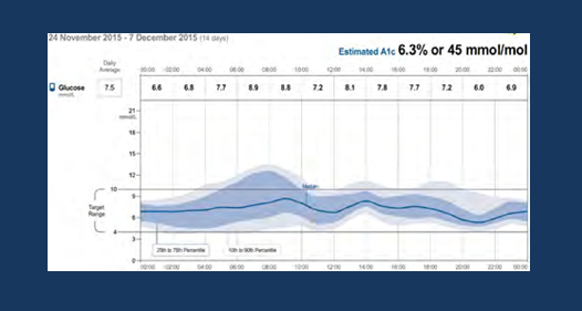
1- slight improvement of the overall stability

2- variability in the morning and before noon suggests improper carb. intake of each meal ;in order to counter this .the patient was advise to mind and reduce their intake ..

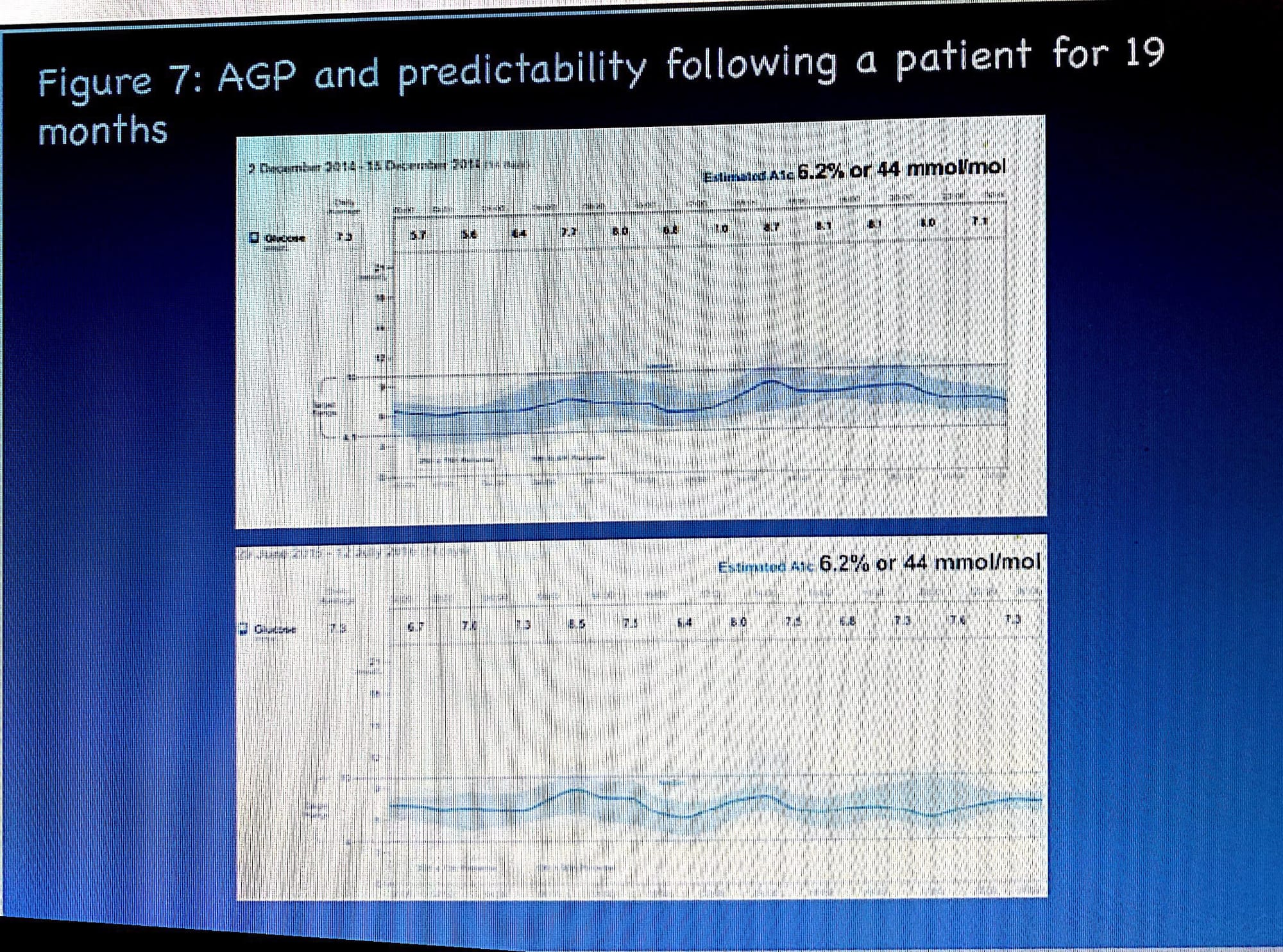
After 18 months lets view the outcome AGP and compare it with the first AGP (reference /baseline /diagnostic) one :

the upper shows ref. AGP and the lower shows last AGP (outcome AGP after successive interventions ) :

1-A1C has been reduced

2-IDR and IQR have been narrowed

3-overall decrease in glucose exposure

4-hypoglycemic risk has been alleviated

5-general improvement of glucose stability and variability

Finally:

The last figure shows the greatness and usefulness (utmost usefulness) of AGP where we can see how was the patient ,what has happened after an intervention and the last outcome AGP, honestly this was unable to be achieved with conventional glucometers .

AGP Analysis in six steps ...

http://ircm.qc.ca/sites/default/files/documents/2018-08/ircm_clinique_outil-pga_en.pdf

FNIR (nice article) also this conccept was discussed recently in in KSA during Medoc 2020 :

FNIR 👇